Following 't Hooft and Veltman one easily obtains the following expression for ![]() :
:
![c0 = Integrate[1/(MandelstamU y) Log[ParticleMass[Pion, RenormalizationState[0]]^2/(MandelstamU y^2 + -MandelstamU y + ParticleMass[Pion, RenormalizationState[0]]^2)], {y, 0, 1}]](../HTMLFiles/index_29.gif)
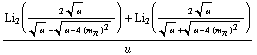
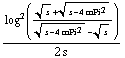
Now, according to the rule (Bürgi): ![]() , we get finally for
, we get finally for ![]() :
:
![c0 = 1/(2 s) Log[((s - 4 mPi^2)^(1/2) + s^(1/2))/((s - 4 mPi^2)^(1/2) - s^(1/2))]^2](../HTMLFiles/index_33.gif)
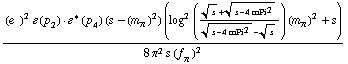
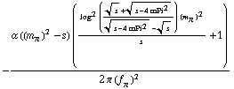
Apart from a factor 2i, the amplitude below is in agreement with Bijnens and Cornet (bugfixed - multiplied with a factor ![]() ):
):
![MandelstamReduce[ampfinalpi0, OnMassShell -> True, Cancel -> MandelstamS, Masses -> {ParticleMass[Pion, RenormalizationState[0]], 0, ParticleMass[Pion, RenormalizationState[0]], 0}] /. {C0[__] -> c0, MandelstamU -> s, -p1 - p2 - p3 -> p4} // Simplify](../HTMLFiles/index_36.gif)
We can now insert some values for the contants and plot the cross section:
![]()
This is then the amplitude to be plotted:
![ampfinalpi00 = MandelstamReduce[ampfinalpi0, OnMassShell -> True, Cancel -> MandelstamS, Masses -> {ParticleMass[Pion, RenormalizationState[0]], 0, ParticleMass[Pion, RenormalizationState[0]], 0}] /. {C0[__] -> c0, CouplingConstant[QED[1], RenormalizationState[0]]^2 -> α 4 π, Pair[Momentum[Polarization[__], ___], Momentum[Polarization[__], ___]] -> 1} /. MandelstamU :> MandelstamS](../HTMLFiles/index_39.gif)
![β[s_] = (s - 4 mPi^2)/s^(1/2) ;](../HTMLFiles/index_41.gif)
![sigma00[ss_, z_] := 1/2 (2 π z)/(64 π^2 ss) β[ss] Abs[2 i ampfinalpi00]^2 /. {MandelstamS :> ss, s :> ss} /. valueRules](../HTMLFiles/index_42.gif)
![]()
![[Graphics:../HTMLFiles/index_44.gif]](../HTMLFiles/index_44.gif)
![]()
![]()
For comparison, here is Bijnens and Cornet's amplitude:
![amp00Bij[s_] := 4 i α 4 π mPi^2 1/(16 π^2 fPi^2) (1 - s/mPi^2) (1 + (s/mPi^2)^(-1) Log[((s/mPi^2 - 4)^(1/2) + s/mPi^2^(1/2))/((s/mPi^2 - 4)^(1/2) - s/mPi^2^(1/2))]^2) ;](../HTMLFiles/index_47.gif)
![]()
![]()
![[Graphics:../HTMLFiles/index_50.gif]](../HTMLFiles/index_50.gif)
![]()
![]()
And here is Holstein, Donoghue and Lin's cross section:
![]()
![]()
![fHol[s_] := 2 (Abs[Log[zPlus[s]/zMinus[s]]]^2 - π^2) + mPi^2/s (Abs[Log[zPlus[s]/zMinus[s]]]^2 + π^2)^2](../HTMLFiles/index_55.gif)
![sigma00Hol[s_] := α^2/(256 π^3 fPi^4) (s - mPi^2)^2/s (1 - (4 mPi^2)/s)^(1/2) (1 + mPi^2/s fHol[s]) /. valueRules](../HTMLFiles/index_56.gif)
![]()
![[Graphics:../HTMLFiles/index_58.gif]](../HTMLFiles/index_58.gif)
All plots agree:
![]()
![[Graphics:../HTMLFiles/index_60.gif]](../HTMLFiles/index_60.gif)
Converted by Mathematica (July 10, 2003)